Selecting a Model
In this post you will learn the basics of computational modeling. Specifically you will learn how to implement a computational model with an example. By the end you will:
- Learn how to select a Model
- Learn how to ammed a Model to suit your needs
- Learn how to implement a decision rule to predict choices in the model
Prerequisites:
- Read through this paper or have some basic background in behavioral economics / learning literature (e.g., reinforcement learning)
- Basic experience in data analysis
My First Model
In order to give yourself a basic working example, I highly reccomend you read through this paper. This is a pretty foundational paper for creating models of decision making and gives a pretty good walkthrough on the process. For example, it describes how/why you typically want to add a noise term when modeling human decisions. Its also quite short, only a few pages.
… Don’t worry I ‘ll wait. 😂
Now that you have finished reading through that, we can go through an example for implementing a computational model on simulated data. The data will be generated from an experiment where the participants need to decide between two lotteries. The lotteries are shown below in the table. I want you to look at each lottery and without looking at the far right column, decide which lottery you would choose: Option A or Option B. Do this for all 10 lotteries.
| Option A | Option B | EV difference |
|---|---|---|
| 1/10 of $2.00, 9/10 of $1.60 | 1/10 of $3.85, 9/10 of $0.10 | $1.17 |
| 2/10 of $2.00, 8/10 of $1.60 | 2/10 of $3.85, 8/10 of $0.10 | $0.83 |
| 3/10 of $2.00, 7/10 of $1.60 | 3/10 of $3.85, 7/10 of $0.10 | $0.50 |
| 4/10 of $2.00, 6/10 of $1.60 | 4/10 of $3.85, 6/10 of $0.10 | $0.16 |
| 5/10 of $2.00, 5/10 of $1.60 | 5/10 of $3.85, 5/10 of $0.10 | -$0.18 |
| 6/10 of $2.00, 4/10 of $1.60 | 6/10 of $3.85, 4/10 of $0.10 | -$0.51 |
| 7/10 of $2.00, 3/10 of $1.60 | 7/10 of $3.85, 3/10 of $0.10 | -$0.85 |
| 8/10 of $2.00, 2/10 of $1.60 | 8/10 of $3.85, 2/10 of $0.10 | -$1.18 |
| 9/10 of $2.00, 1/10 of $1.60 | 9/10 of $3.85, 1/10 of $0.10 | -$1.52 |
| 10/10 of $2.00, 0/10 of $1.60 | 10/10 of $3.85, 0/10 of $0.10 | -$1.85 |
Selecting a Model
The first and most important part for computational modeling is the model that you select. You should definitely take some time when selecting a model because this IS YOUR PREDICTION for how participants will make decisions in experiment. Often times you will use a model that has already been used in other experiments, but occasionally, you will need to make your own (or much much more likely, you will have to adjust an existing one). With that in mind, I will go through a really basic example for adjusting models to improve them. This should give you a sense of how this process works, such that you can do it on your own when the time requires it.
Our example (simulated) data is going to come from people making choices between different lotteries involving money. As such, expected value (EV) is definitionally, an optimal starting point. For the uninitiated, EV is a mathematical formula for determining the value of a risking lottery. So if you are acting perfectly rationally, you should choose the lottery with the highest EV. The formula for EV is:
\[EV = \sum_{i=1}^{k} p_i \times v_i\]where $p$ is the probablity of winning the lottery and $v$ is the value that you get if you win that lottery. $k$ represents the total number of options for the lottery. So if you have a lottery that was 50:50 and if you win you get $10 and if you lose you get $0 then you could solve with:
\[EV = .5 * 10 + .5 * 0\] \[EV = 5 + 0\] \[EV = 5\]Another way to say this is if you played this lottery an infinite number of times, we would expect you to, on average, earn $5. This should make intuitive sense giving the options of the lottery. This formula is useful because it works no matter what the probabilities or winning amount are, and it doesnt matter how many of them their are.
We can apply that same formula to all the lottery options shown in the table above. And then we will take the difference in EV between the two options (see right most column). Finally, we can implement a decision rule, that is a rule to decide which option to pick. For EV, you should pick the option that has a higher expected value. In the figure below, we plotted the probability of choosing the first option (Option A) for each of the 10 lotteries, given our model/decision rule combo.
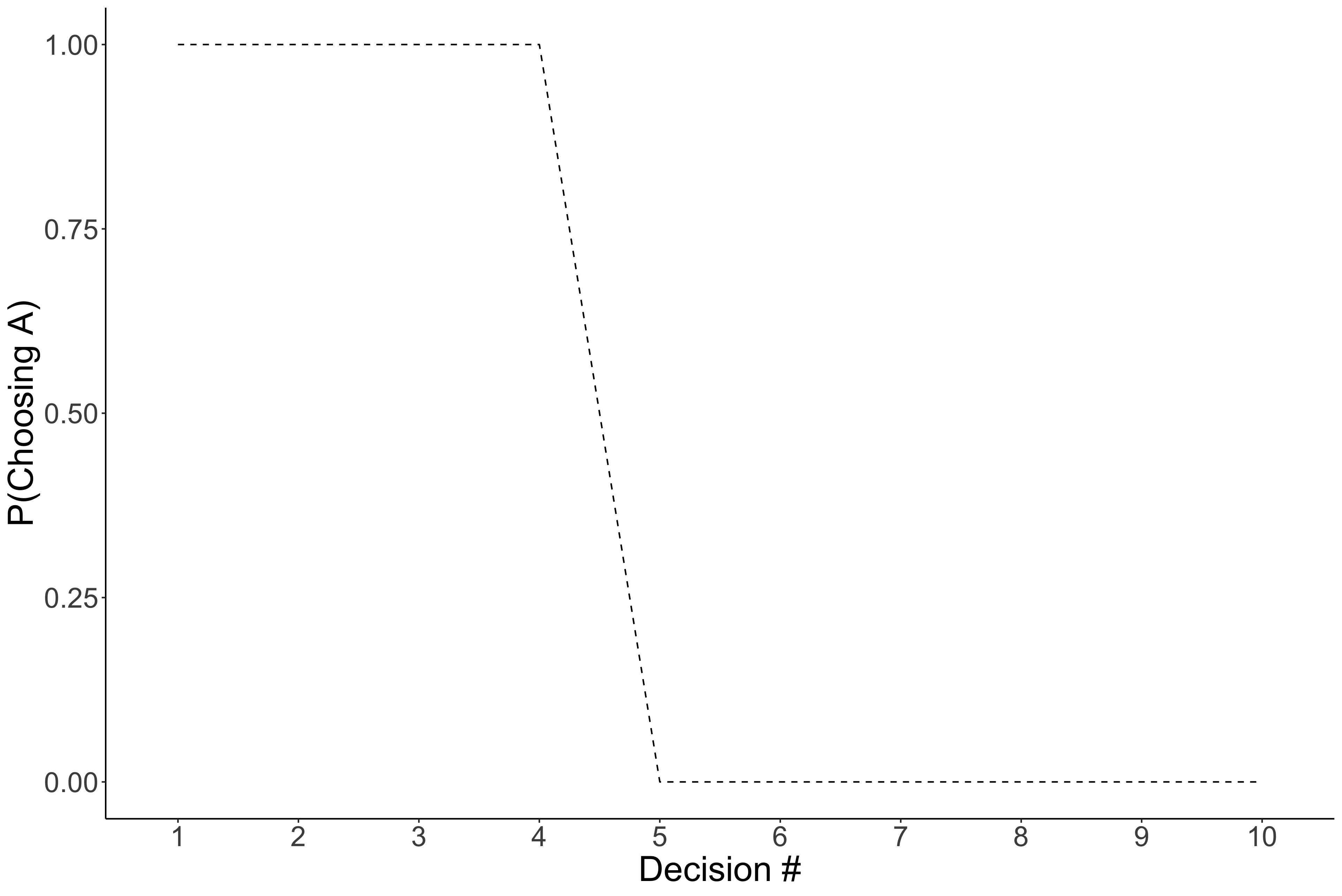
Notice that this model predicts that people would select option A for the first 4, and then select B for the remaining ones. As described above, this is mathematically optimal. But the question is, how would you expect people to decide to their lotteries? Which did you choose when you picked between them?
Here is some simulated data to use as a comparison:
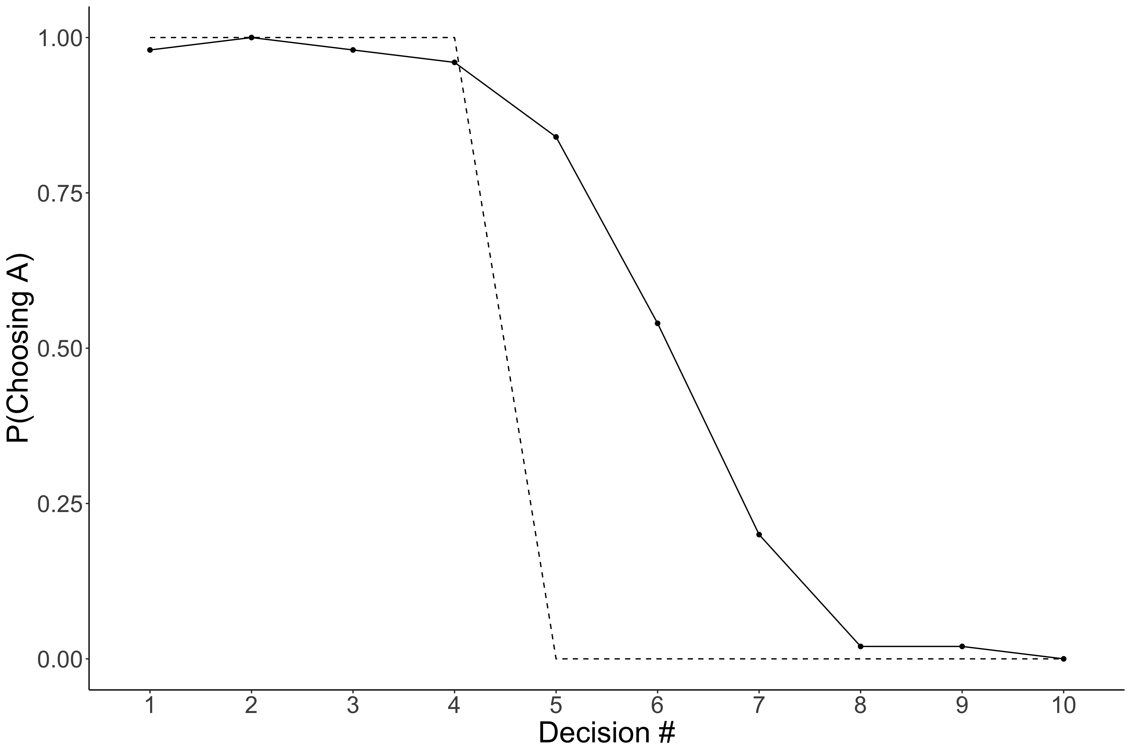
Again the dotted line indicates the EV models predictions, and the new solid line with dots indicates the average response for 50 simulated people. What are your thoughts? Is this model any good? You might think, no, its pretty bad, which it is…, but there are some important things that it gets right. Notice that the simulated data has a similar structure as the prediction. That is, pretty much everyone chooses Option A for the first 4 and everyone selects Option B for the final 3. So in reality, it only gets the middle ones wrong. So maybe we can adjust this model to account for that as opposed to come up with an entirely new model.
A Story of Individual Differences: Adding Parameters
One thing you might have noticed, is that the EV model expects everyone to make the same choices. The hypothesis is so absurd that is can be rejected outright. Instead, it is pretty obvious that people make different choices; for example, some people really don’t like it if the odds of winning are not in their favor. In Psychology/Econoimics, we call this behavior risk aversion. And we can add this to the model as well. Continuing with our example, this can be done by adding a exponent to the $v$ term in EV. For example:
\[SV(p, v) = \sum_{i=1}^{k} p_i \times v_i^{\alpha}\]There are a few things I want to point out. First I changed the function from $EV$ to $SV$. This is to signify, that this is no longer an equation for expected value, but rather, for subjective value, or the value an individual places on that lottery. The second is that I have made it more clear that $p$ and $v$ are inputs to the model by including them in the parentheses on the left side. Finally, you can see the new term $\alpha$ (pronounced alpha) which is unique to each individual.
The new parameter ($\alpha$) allows us to be able to predict that people will make choices different from one another; however, importantly, we expect everyone to make choices with this specific structure in mind. So, although people differ on what they consider a reasonable lottery, we expect them to weigh the probability by the amount they could win. The $\alpha$’s allow us to adjust for each person what their specific threshold is for what makes a good lottery. While this is a bit simplified, hopefully it gives you a general intuition for the formula. For simplicity and ease of understanding, we will use a single $\alpha$ for the whole groups average decision, but the same process would work for each individual.
Note: Traditionally, individual specific parameters typically use greek letters. This can help you identify what parts of the model is an input versus participant specific.
Now we can use this model to predict the participant’s decisions. But which $\alpha$ should we use? Well since we are just exploring, let’s pick a few to see which ones look more accurate. Since we are plotting the average data, these plotted $\alpha$’s are really a meteric of the average $\alpha$.
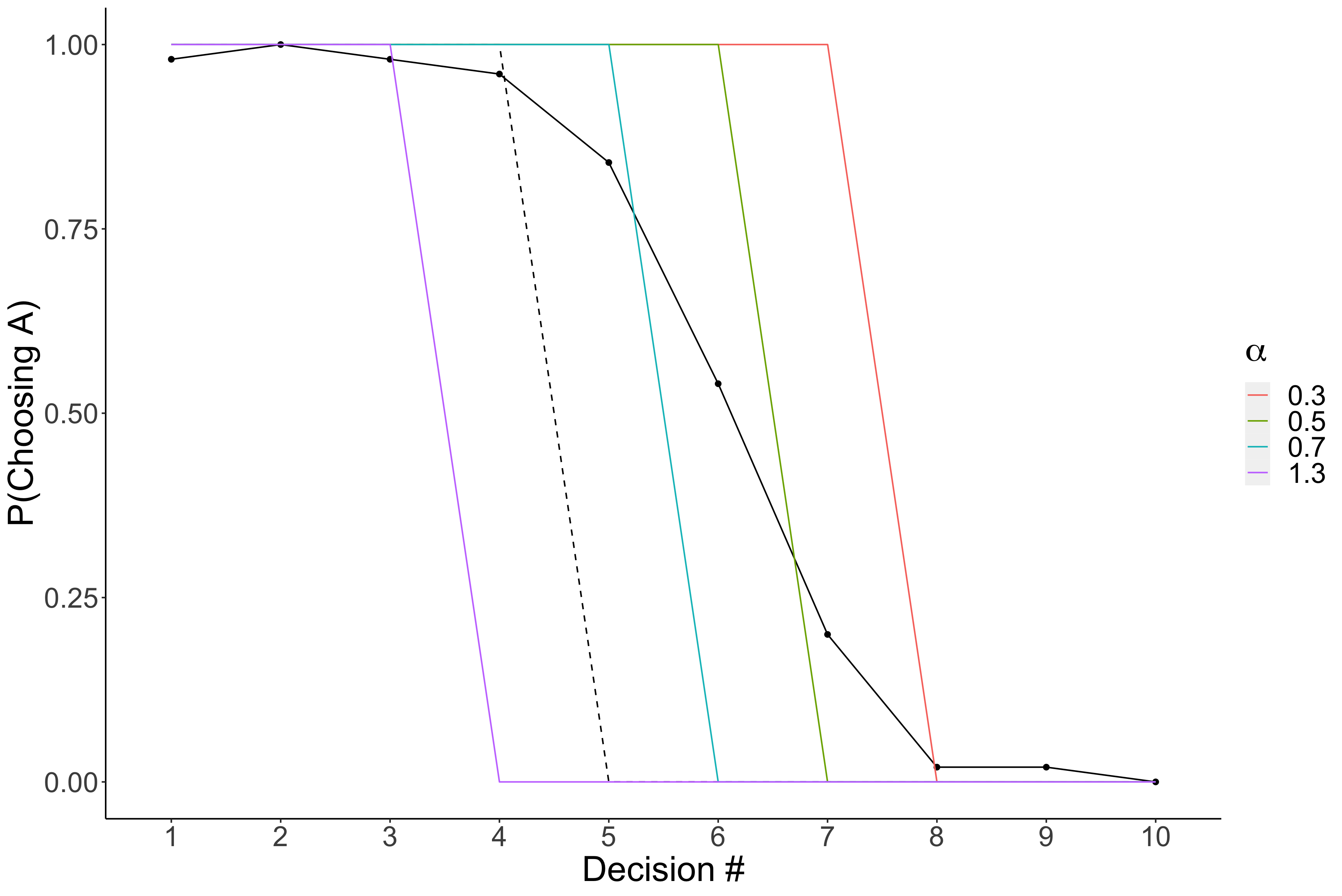
Now we added the colored lines. What you should notice is that it seems like that blue (.7) and green (.5) lines seem to improve on the EV model in that it gets the threshold a littel bit more accurate. This is a good sign. It lets us know we are on the right track.
Note: These are simulated data and not necessarily representive of real data. Some values have been intensionally exaggerated for pedogological reasons.
But there is something still bothering me, and hopefully you as well. The thresholds are really sharp; the data has a gradual decline as a opposed to be completely instantaneous. Let’s fix that by adjusting the decision rule.
Decision Rules
We are going to add another equation to serve as a rule for making the choice. So instead of simply choosing the option with the higher EV or SV we will have a more graded response. As with most things, there are a few different equations you could use. For this tutorial, we will use an inverse logit function:
\[p(Option_A\mid SV_a, SV_b) = \frac{1}{1 + e^{\gamma(SV_b - SV_a)}}\]Here, the function is for the probability of choosing option A for a particular lottery (the probability of choosing option B is just $1-p$). And to calculate this probability, you need the subjective value for both option A ($SV_A$) and B ($SV_B$), which implies we also need that person’s $\alpha$ to calculate their $SV$’s. Additionally, you see $e$, which is the mathematical constant $\approx$ 2.7. Finally, we introduced a new parameter $\gamma$ (pronounced gamma). This is commonly described as a noise term because it allows for people to be noisy in their decisions, in other words they are not always consistent meaning you will get that graded response seen in the black solid line.
But again we have an issue, what is the correct $\gamma$? Of course, without looking at the data you would be hard pressed to give a sensible answer. So we will use a similar stragey, use a couple and plot them.
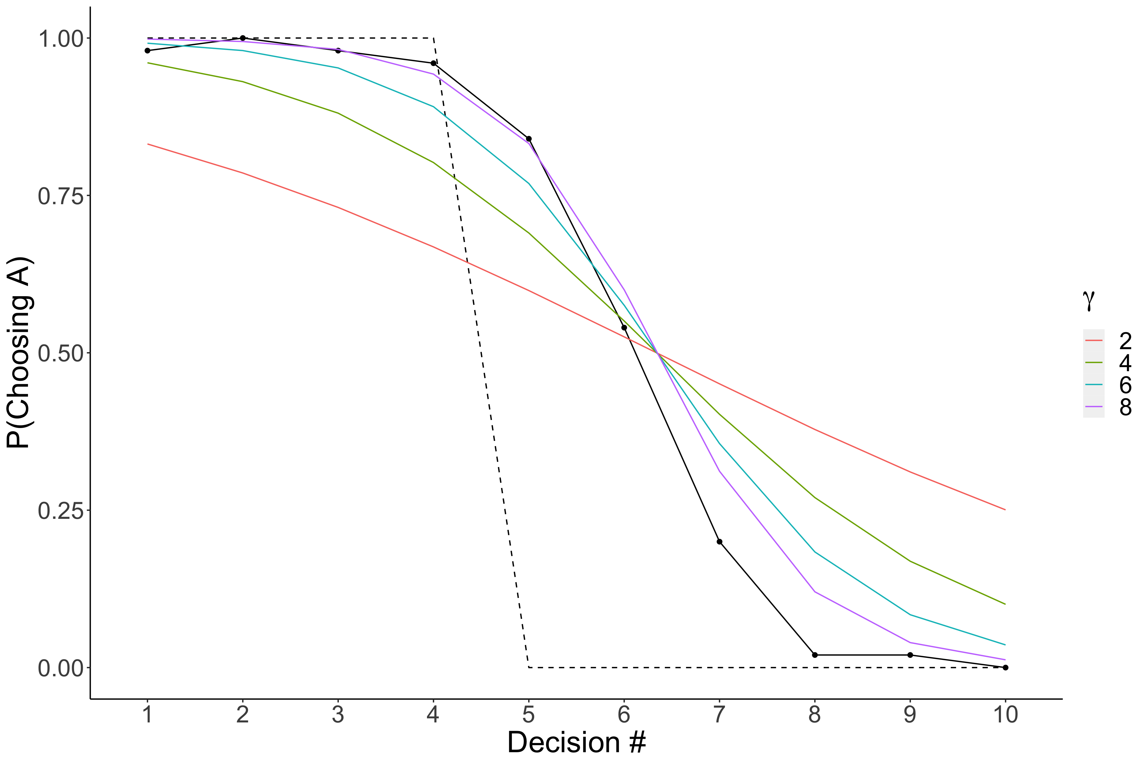
This looks incredible!! We are having very close predictions to the real data! Specifically, when $\gamma=8$ it seems to match the data really well.
Recap
Now that you got the hang of what a computational model is and how they work, you are ready for the next section. In the next tutorial, you will dive deeper into computational models. Specifically, you will learn how to estimate the parameters of your model instead of guessing and checking. Additionally, you will learn how to evaluate whether its a good model or not.